Sat-Sun: Non-working days
Project Objective: To develop an efficient volumetric modeling methodology for the N deposit (commercially sensitive) for use in applied geological research.
As part of the project for the Client (commercially sensitive), block, skeletal, and triangulated 3D models were created.
Project Results:
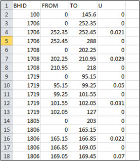
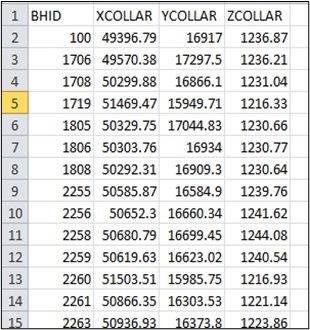
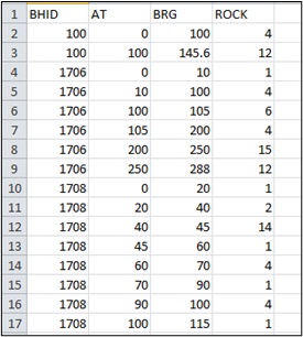
To calculate the reserves and resources of this deposit, we were provided with a database including assay results, inclinometry measurements, and well coordinates. All information was contained in the following files.
|
|
| Figure 1 Structure of file ‘assay.csv’ | Figure 2 Structure of file ‘collar.csv’ |
In the "assay.csv" file, assay results of ore bodies were provided (Figure 1). In the "collar.csv" file, coordinates of all boreholes were contained (Figure 2).
|

|
| Figure 3 Structure of file ‘geology.csv’ | Figure 4 Structure of file ‘survey.csv’ |
In the "geology.csv" file, information regarding the lengths of all boreholes was provided (Figure 3). In the "survey.csv" file, information about borehole deviation was contained (Figure 4).
In the "topo.csv" file, elevation measurements tied to x and y coordinates, provided by the surveyor, were included (Figure 5).
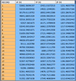
Figure 5 Structure of file ‘topo.csv’
Using the file from the surveyor's surface survey, a framework for the topo-surface (DTM – Digital Terrain Model) was created. Using specific commands in Datamine Studio3, we integrated the files "assay.csv," "collar.csv," "geology.csv," "survey.csv," and "topo.csv" into a single file, which opened in the program as a three-dimensional model of boreholes (Figure 6).
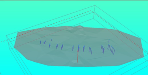
Ris. 6. Three-dimensional model of the surface and boreholes of deposit N in Datamine Studio 3.
1. Framework modeling.
The outlines of ore bodies were delineated based on assay sections, as the modeling in this case was conducted solely based on geological characteristics rather than economic parameters.
Subsequently, we constructed contours of component concentrations based on these composites (Figure 7).
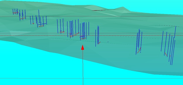
Figure 7. Contours of ore bodies across sections.
Based on these contours, the framework of the main ore body and lenses above it was created (Figure 8).
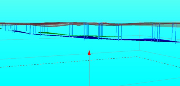
Figure 8. Framework of the main ore body and lenses above it.
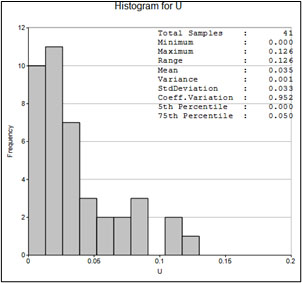
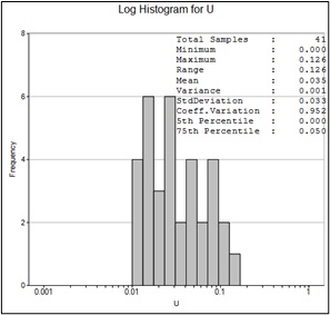
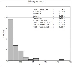
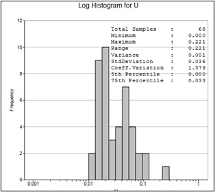
Next, all samples inside the ore body and lenses were extracted into a separate file. Based on the assay results of the ore bodies, histograms were constructed, and statistical characteristics were obtained (Table 1).
|
|
| Figure 9. Histogram of valuable mineral distribution in the main ore body | Figure 10. Histogram of valuable mineral distribution after logarithmic transformation in the main ore body |
|
|
| Figure 11. Histogram of valuable mineral distribution in lenses | Figure 12. Histogram of valuable mineral distribution after logarithmic transformation in lenses |
Analysis of the histograms shows that the distribution of valuable minerals (commercially sensitive information) follows a lognormal distribution (Figure 9 - 12).
Table 1. Statistical indicators of valuable mineral distribution
| Number of Samples | Minimum | Maximum | Mean | Variance | Coefficient of Variation | Quantile Spread | |
| Main Ore Body | 41 | 0 | 0.126 | 0.035 | 0.001 | 0.952 | 0.05 |
| Lenses | 68 | 0 | 0.221 | 0.026 | 0.001 | 1.379 | 0.033 |
2. Construction of Block Model of Ore Bodies
First, a prototype model was created, for which the size of the elementary block was determined (103 cubic meters). The distance between profiles was 200 meters, and between wells along the profile was 50 meters. However, this size of the elementary block was chosen based on the small thickness of the main ore body and overlying lenses. To ensure that the volume of ore bodies was fully filled, sub-blocks were created. For this purpose, the splitting coefficient of the parent block was chosen as average. An attempt was made to conduct variogram analysis to analyze the variability of valuable mineral contents in the ore body of the deposit. However, due to the small number of samples characterizing the ore body and lenses, this was not successful. Therefore, interpolation of valuable mineral distribution into elementary blocks of ore body models and lenses was carried out using inverse distance weighting and nearest neighbor methods.
3. Interpolation
The task of interpolation is to forecast the distribution of valuable mineral contents within the blocks of the created model based on the contents in samples from exploration wells located within the block model. For the interpolation procedure, we used the Estimate process in Datamine Studio 3. After entering the names of the files for the empty block model and the well file into the process menu, the sizes of the search ellipsoids for samples were inputted (Table 2, 3).
Table 2. Dimensions of Search Ellipsoid Axes
| Axes | Dimensions of 1st Ellipsoid | Dimensions of 2nd Ellipsoid | Dimensions of 3rd Ellipsoid |
| X | 10 | 20 | 120 |
| Y | 10 | 20 | 120 |
| Z | 10 | 20 | 120 |
For interpolation, it was decided that each well would utilize only 2 samples, and the minimum and maximum number of samples for interpolation are specified in each ellipsoid in Table 3.
Table 3. Number of Samples Used for Model Interpolation
| Minimum Number of Samples | Maximum Number of Samples | |
| 1st Search Ellipsoid | 1 | 20 |
| 2nd Search Ellipsoid | 1 | 20 |
| 3rd Search Ellipsoid | 1 | 20 |
As mentioned earlier, interpolation was performed using two methods: inverse distance weighting and nearest neighbor method. A power of 3 was used for the inverse distance weighting interpolation. Interpolative estimation of valuable mineral contents was conducted for each sub-block due to the small size of the ore body and lenses.
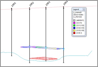
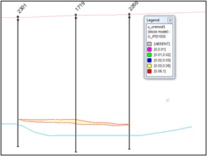
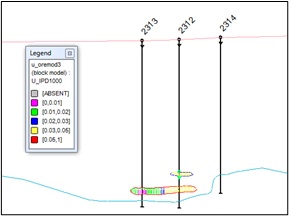
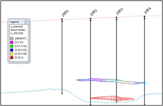
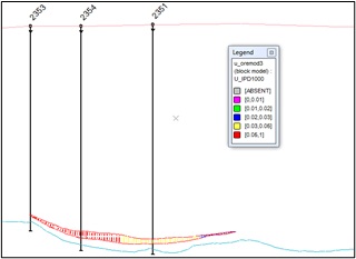
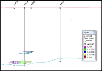
Below, in Figures 13 and 14, the distribution of valuable mineral contents in the block model of the main ore body and lenses is shown (Figure 13).
|
|
|
|
|
|
fig. 13. Mineral distribution sections in a block model of the main ore body and deposit
<tbody>
<tr>
<td>
<img width="326" alt="14 а.jpg" src="/upload/medialibrary/567/14_a.jpg" height="212" title="14 а.jpg">
</td>
<td>
<img width="293" alt="14 б.jpg" src="/upload/medialibrary/515/14_b.jpg" height="214" title="14 б.jpg">
</td>
</tr>
<tr>
<td>
<img width="298" alt="14 в.jpg" src="/upload/medialibrary/b6a/14_v.jpg" height="200" title="14 в.jpg">
</td>
<td>
<img width="321" alt="14 г.jpg" src="/upload/medialibrary/c81/14_g.jpg" height="198" title="Рис.14. Разрезы распределения полезного ископаемого в блоковой модели главного рудного тела и линз месторождения ">
</td>
</tr>
</tbody>
</table>
<p>
Fig. 14 Mineral distribution sections in the block model of the main ore body and lenses of the deposit
</p>
4. Calculation of reserves based on geological data
In this study, the calculation of reserves based on geological data and assay results was conducted for the first time using three-dimensional modeling.
The reserves calculation of the model was performed based on the ore grade.
The results of the reserves calculation are confidential.


